INTRODUCTION
Flame characteristics have long been a subject of interest in fire safety because the size and shape of the flaming region and plume affect fire spread. Flaming region characterization is useful in building design, safety protocol development, and in the area of fire forensics. Estimating flame height and direction can help fire investigators determine how fire spreads from one object to others and therefore supports reconstructing fire scenarios.
Wind or airflow caused by doors and/or windows in the case of compartment fires can cause a flame to tilt. Simple flame height correlations do not account for this phenomenon. In compartment fires especially, flame tilt is important because it may cause an object located in the direction of the tilt to ignite and lead to secondary ignition. Nonetheless, flame tilt is often not incorporated into fire spread models. This is the case in B-RISK, a fire risk assessment tool that features a point source sub-model capable of predicting ignition times for combustible items within a compartment during a fire. Sazegara et al [1] presented an analysis of the B-RISK predictions compared to experimental measurements and noted that flame leaning caused inaccuracies in the B-RISK predictions. Buffington et al. [2] used Bayesian inference and a machine learning framework to infer radiative fraction in pool fires. Their Bayesian framework used a point-source model, which they adjusted due to inaccuracies caused by flame leaning.
Given the importance of flame tilt in fire spread, the ability to estimate flame position for ventilated compartment fires is crucial. In applications where many predictions are needed, high-fidelity software is prohibitively expensive, and conducting experiments for each scenario is not feasible. Therefore, developing lower-order models which can make predictions in seconds or less is important. The primary objective of this project is to develop a low-order model based on machine learning to characterize the effects of vent flows on pool fires in compartment fires. The proposed framework uses a transpose convolutional neural network that predicts the spatially resolved heat release rate per unit volume (HRRPUV) in a compartment based on inputs describing fire size, location, and ventilation conditions. The model is trained on data generated using the Fire Dynamics Simulator (FDS). The spatially resolved HRRPUV is then used to extract the coordinates of the centerline of the flame.
TRAINING SET
The training set was generated using FDS version 6. Inputs to the model were randomly selected from uniform distributions. Room width and length were drawn from uniform distributions with bounds 2.5 and 9 m. The ceiling height was 2.6 m for all simulations. A fully open door of width 1 m and height 1.8 m was placed on one wall (the same wall in all simulations). Its location on the wall was randomly drawn from a uniform distribution ranging from 0 m to the width of the room drawn minus 1 m (to accommodate for the door width, which was 1 m). A burner of size 0.4 x 0.4 m was placed in the room. The x and y coordinates for the center of the burner were drawn from uniform distributions with bounds depending on the room width and length previously drawn. Figure 1 shows the simulation domain for one simulation. The (steady) heat release rate (HRR) was randomly drawn from a uniform distribution with bounds 100 and 1000 kW. The grid cell size was set to 0.2 m and the fuel used was propane. Twelve horizontal slices recording heat release rate per unit volume (HRRPUV) were defined; one every 0.2 m starting at 0.4 m. In total, 2,867 simulations were run. The simulations were run for 150 s. The HRRPUV slices were averaged over the last 50 s of the simulations. The data generated were split between training and testing datasets. The testing dataset was set aside and later used to evaluate the performance of the model on simulations that were not used during training.

Figure 1. Simulation domain for a given simulation.
EXTRACTING FLAME CENTERLINE COORDINATES
For each horizontal HRRPUV slice, the flame center coordinates were calculated using:

The z location corresponds to the height of the slice. As an example, Figure 2 shows the twelve time-averaged HRRPUV slices and the position of the flame centerline at each z location for one FDS simulation. As z increases, flame tilting becomes apparent (the burner position and center point differ). In addition, flame height was also estimated using HRRPUV slices. Flame height was defined as the z location where the cumulative HRR is closest to 90% of the total HRR.

Figure 2: plots showing HRRPUV as a function of height. The burner center and flame center are shown.
MODEL
The machine learning model used is very similar to the one used by Hodges et al. [3]. Hodges et al. used a convolutional neural network to predict spatially resolved temperatures and velocities in compartment fires. Instead of predicting temperatures and velocities, the present study uses the model to predict HRRPUV. From the HRRPUV predictions, the flame centerline coordinates are extracted as detailed above. A visual representation of the model is shown in Figure 3 (taken from [3]).
For each prediction, the model outputs twelve slices of 50x50 values, hence the 50x50x12 output shape. The inputs to the model consist of 1) the inputs given to FDS and 2) zone layers model inputs. The FDS inputs comprise of: HRR, burner location (x and y), room width and height, and door location. Zone model inputs were added to provide additional information to the model. Zone layer models assume that the compartment is divided into two or more layers of uniform properties. CFAST is an example of a zone model. Hodges et al. [3] used zone model inputs for their model. As a first step, they extracted the zone layer inputs directly from the FDS simulations rather than from secondary zone model (such as CFAST) to ensure that no secondary source of error was introduced to the model. They then iterated on their model and calculated zone layer inputs using CFAST.
At this stage of the project, the first method was used: zone layer inputs were extracted from the FDS simulations themselves, using the equations provided by Hodges et al. [3] along with density, temperature and velocity slices placed at the door in FDS. In future iterations, CFAST will be used instead. The zone model inputs used were upper and lower layer temperature, upper and lower layer mass flow rate through the door, height of the neutral plane, and height of the interface plane. The input shape to the model was therefore a vector of 12 elements (6 initial inputs + 6 zone model inputs.)
The model was built using Keras in the Python library Tensorflow. It was trained for 500 epochs with early stopping.

Figure 3: Figure showing the architecture of the model (taken from Hodges et al. [3])
RESULTS
The performance of the model was evaluated by comparing predictions made for the test dataset inputs and the known, “true” outputs. There were 144 simulations in the test dataset. Figure 4 shows histograms for two metrics for evaluating the model: root mean squared error (RSME) between the true and predicted HRRPUV and mean distance between the true and predicted centerline (one value in the histogram corresponds to one simulation). The mean RSME across simulations was 8.62 kW/m3, and the mean for the mean absolute distance between the true and predicted centerlines was 0.16 m.

Figure 4: plots showing distributions for RSME for HRRPUV (left) and mean absolute distance between true and predicted centerlines (right).
Figure 5 shows predicted flame height against true flame height. The closer the points are to the gray line, the better the predicted and true flame heights agree. Note that some points overlap. The mean difference between the predicted and true flame heights was 15 cm, which is smaller than the length of the sides one grid cell (20 cm).
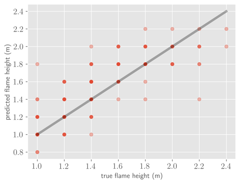
Figure 5: Plot showing true flame height against predicted flame height for all 144 test cases.
Figure 6 shows the predicted and true centerlines in the x-z and y-z planes for a single test case, and Figure 7 shows a top view of the flame centerline for the same case. The color gradient in Figure 7 shows the points’ height.
 Figure 6: plots showing the true and predicted centerlines in the x-z plane (left) and y-z plane (right).

Figure 7: plots showing the true (left) and predicted (right) centerlines in the x-y plane. The color gradient represents height.
CONCLUSION AND FUTURE WORK
A machine learning model was built to predict flame height and position based on compartment and ventilation characteristics. The model was tested on 144 FDS cases that were not used in the training process. Future work will involve using CFAST as opposed to FDS to calculate zone layer inputs and re-assessing the model performance after this change. Future iterations will also account for door (or window) size, which was not done in the most current version of the model. Finally, the model will be used to inform a point-source model and to compare predictions to data collected by Buffington et al. [2].
REFERENCES
[1] Sazegara, S., Spearpoint, M. and Baker, G., 2017. Benchmarking the single item ignition prediction capability of B-RISK using furniture calorimeter and room-size experiments. Fire technology, 53(4), pp.1485-1508.
[2] Buffington, T., Cabrera, J.M. and Ezekoye, O.A., 2022. Statistical aggregation of heat flux measurements for Bayesian inference of a burner fire's radiative fraction. Fire Safety Journal, 129, p.103559.
[3] Hodges, J.L., Lattimer, B.Y. and Luxbacher, K.D., 2019. Compartment fire predictions using transpose convolutional neural networks. Fire Safety Journal, 108, p.102854.