europeissue40feature1

Calibrating a 1D Tunnel Ventilation Model Using Real-World Data and AI Techniques: Application to a Large Urban Network

By: Fabián de Kluijver, JVVA, Spain, Alberto López, JVVA, Spain

Juan Manuel Sanz, Sener, Spain, Guillem Peris, Sener, Spain

Javier Berges, Madrid Calle 30, Spain, Mar Martinez, Madrid Calle 30, Spain

The present article offers a condensed synthesis of work previously presented at the 12th Tunnel Safety and Ventilation Conference (2024) [1], where the complete AI-supported field-data analysis and calibration workflow was described, and later in NAFEMS Benchmark magazine (July 2025) [2], which focused on the surrogate-modeling and calibration process.

1. Introduction

Ventilation design in road tunnels is essential for fire safety. During fire events, controlling smoke movement, maintaining tenable conditions for evacuation, and supporting firefighting operations depend on accurately predicting airflow under different operational and environmental conditions. In large infrastructures, this understanding relies increasingly on computational models, which must be carefully calibrated to reflect real behavior.

This article summarizes the calibration of a one-dimensional (1D) ventilation model for Madrid’s M30 tunnel network, one of Europe’s largest and most complex urban tunnel systems. The scale and heterogeneity of the network introduce uncertainties inherent to any physical model, making calibration a critical step. The availability of extensive field data provided a strong basis for refining predictions and reducing these uncertainties. To accomplish this, the project combined traditional engineering models, surrogate modeling, and artificial intelligence (AI) tools for data analysis. The resulting calibrated digital twin supports the development of both sanitary and fire ventilation strategies. Although centered on the M30, the methodology is applicable to other complex infrastructures where manual calibration is not feasible.

2. A Complex Urban Tunnel System

The M30 tunnel network forms a continuous underground ring around central Madrid. It includes 48 km of tunnels, equivalent to 118 km of single-lane roadway, with daily traffic exceeding 1.3 million vehicles. The system incorporates 21 entrances, 22 exits, branching points, and widely varying cross sections. All of these elements contribute to a complex ventilation behavior resulting from the interaction between multiple interconnected tunnels.

The scale of the ventilation infrastructure further illustrates the system’s complexity. As shown in Figure 1, the network includes nearly 1,000 ventilation fans and 684 environmental sensors, including 388 anemometers. This inventory shows the diversity of ventilation systems across the network, while the sensor deployment provides the monitoring capability needed for model calibration.

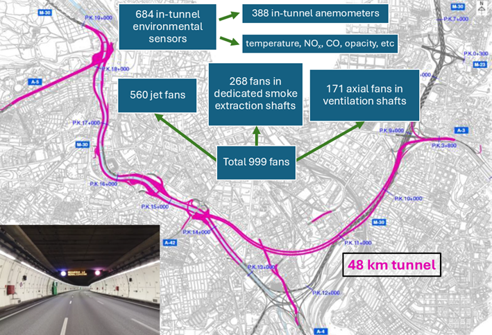
Figure 1. Map of the tunnel network, and list of tunnel ventilation equipment and air quality monitoring sensors.

3. Motivation and Objectives

With the tunnel’s ventilation control equipment having reached the end of its useful life, a renewal project was started to ensure continued compliance with operational and safety requirements. This upgrade also provided an opportunity to reanalyze the existing ventilation approach and update the corresponding control algorithms. Improving these algorithms required an accurate understanding of airflow behavior under a wide range of operating conditions, motivating the development of a calibrated 1D ventilation model for the entire network.

Although three-dimensional fire simulations using Fire Dynamics Simulator (FDS) software were also conducted, these are limited to analyzing smoke movement in localized zones under predefined boundary conditions. They cannot represent the system-wide aerodynamic response to different equipment activation scenarios. A 1D model, on the other hand, can capture global flow balances, pressure losses, heat transfer effects, and interactions between ventilation equipment across the full network. The main objective of this work was therefore to develop and calibrate such a model using field data.

4. Preparing and Understanding Field Data Through AI

Processing the M30’s field data required a dedicated methodology. Over the last decade, more than three terabytes of operational data have been recorded by the control center, including traffic information, anemometer readings, environmental measurements, and equipment states. The scale and heterogeneity of this dataset made manual processing unmanageable, requiring the use of AI-assisted tools.

The first step was data homogenization, removing periods not representative of normal operation such as fire drills, equipment faults, or sensor malfunctions. AI routines compared each sensor to its neighbors to detect anomalies and improve dataset consistency. Clustering and pattern-recognition techniques then grouped anemometers with similar temporal behavior, revealing aerodynamic zones within the network and providing a clearer understanding of how different areas respond to traffic, natural draft, and thermal conditions.

AI analysis also quantified relationships between traffic flow, vehicle speed, and air velocity, clarifying the role of the piston effect. Temperature records showed how natural draft relates to external weather, influencing airflow direction and magnitude. In addition to cleaning and characterizing the data, these AI-based methods provided valuable tools for visualizing and analyzing ventilation behavior across different areas and operating conditions, improving the system-level understanding needed to interpret field data for model calibration.

5. The One-Dimensional Ventilation Model

The ventilation model was implemented using IDA-Tunnel [6], a simulation tool widely used in the design of railway and road tunnel networks around the world, and validated through several studies [7], [8]. A 1D model is appropriate when longitudinal dimensions far exceed transverse ones: flow variables vary along the tunnel axis but are assumed uniform across each cross section. Although simplified, this approach effectively models the global airflow behavior at reduced computational cost, including fluid phenomena such as pressure losses, vehicle-induced piston effects, pollutant transport, and thermal influences.

The M30 tunnel network model comprises 194 interconnected tunnel segments between portals, branches, and connections to ventilation shafts, as illustrated in Figure 2. Depending on the sector, the model represents longitudinal, transverse, or semi-transverse ventilation, reflecting the ventilation configurations present in the infrastructure.

For this study, the simulation model inputs are grouped into two categories:

· Model parameters (θ): inputs to the model that remain constant over time and whose values carry an associated uncertainty. In this study, these parameters include friction coefficients, representative cross-section heights, vehicle aerodynamic coefficients, and a wall-temperature-related parameter introduced to compensate for steady-state simplifications.

· State inputs (x): time-varying quantities measured in the field. In the model considered, these inputs correspond to traffic flows in each tunnel segment and the ambient temperature. For this study, they are assumed to be known from field data, and no uncertainty is assigned to them.

Calibration focused on determining the values of the model parameters (θ) that minimized the discrepancy between simulated and measured air velocities across the network’s anemometers.

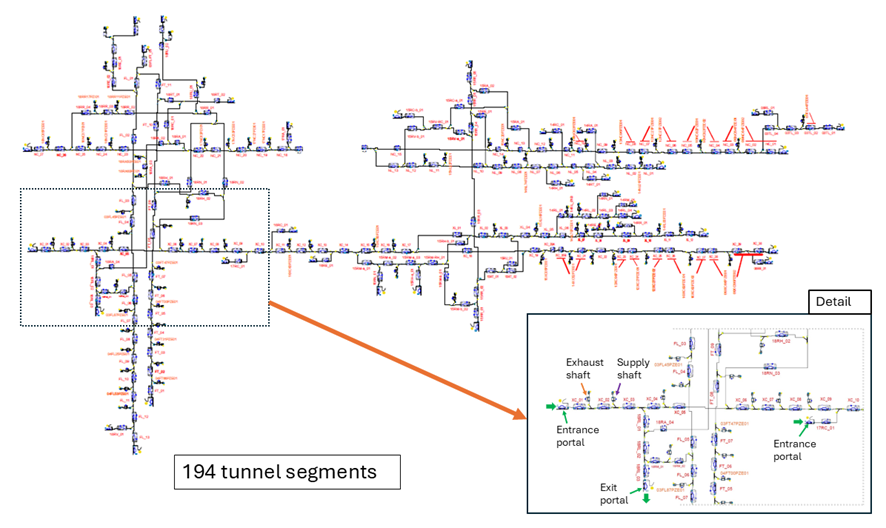
Figure 2. Diagram of the 1D simulation model.

6. Calibration Methodology

6.1 Calibration Framework

Some of the available field data correspond to state inputs of the model, such as traffic flow and ambient temperature. Other variables measured in the field correspond to model outputs, including air velocity at different anemometers and temperature within the tunnels. This relationship between model inputs, model outputs, and the available field data is illustrated in Figure 3.

Assessing how accurately the model reproduces real airflow behavior requires a systematic method. In this study, air velocity is selected as the output variable for calibration, since it is measured throughout the network by hundreds of anemometers and provides a direct indicator of the system’s behavior. For each combination of model parameters (θ) and state inputs (x), the 1D model generates predicted air velocities at all anemometers. These predictions are compared with field measurements, producing error values across a wide range of operating states. Individual errors are then combined into a global error metric that depends only on θ.

The calibration process consists of an optimization process that aims to find the θ values that minimize this metric. To carry out this task, the calibration process needs to explore the parameter space by comparing simulation outputs with field data across many different combinations of model parameters and state inputs. This exploration seeks the parameter set that provides the best overall agreement with the measurements. Since such an extensive search cannot be performed manually, an automated method is required to efficiently evaluate and refine candidate parameter sets. Achieving this relies on an iterative optimization procedure in which successive candidates are tested and progressively improved until the convergence criteria are met. In this project, a differential evolution algorithm [3] was selected for the optimization process because of its ability to explore high-dimensional parameter spaces effectively and avoid convergence to local minima (global optimization). An overview of this iterative process and its structure within the calibration workflow is shown in Figure 4.

For the calibration, the focus was placed on periods without mechanical ventilation, when airflow is driven only by traffic (piston effect) and thermal differences (natural draft). To ensure that only these natural-ventilation conditions were used, field data corresponding to any hour in which jet fans or extraction shafts were active was filtered out. The dataset used for calibration covered an entire year of measurements, specifically the most recent full year available: 2021, which contains 8,760 hours of recorded data. After removing all periods with active ventilation equipment, a total of 3,884 hours remained. Each of these hours was treated as a quasi-steady-state period in which traffic flow and ambient temperature were assumed constant, allowing the calibration to focus on average system behavior rather than transient effects. Although no two hours present exactly the same traffic and temperature values, the system state tends to repeat in an approximate manner throughout the year, giving rise to groups of state input vectors that are very similar and can be expected to induce similar airflow conditions in the tunnels. For this reason, these hours were grouped into 500 representative clusters in order to preserve variability while reducing computational load during the optimization process.

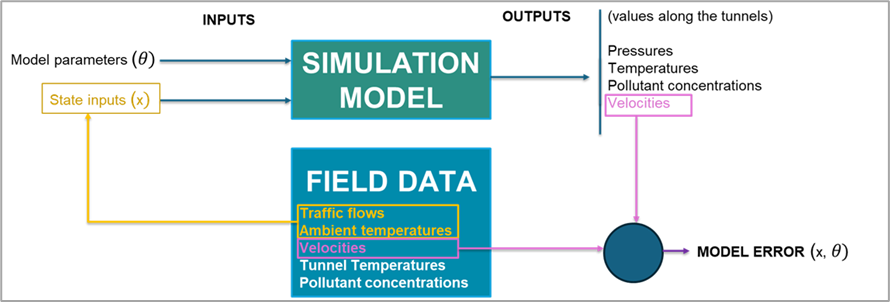
Figure 3. Diagram of relationships between model inputs, model outputs, field data, and calculation of model error.

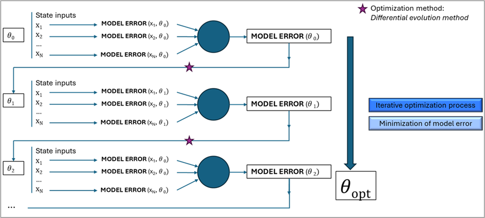
Figure 4. Diagram of calculation of global model error and representation of the calibration process as an iterative optimization method over the parameter vector.

6.2 Computational Cost and Surrogate Modeling

Taking into account that each 1D simulation requires approximately 20 seconds and that each optimization iteration needs to evaluate 500 representative operating states, a single iteration of the calibration process would take roughly 2.8 hours to complete. Since an optimization process of this type typically requires hundreds of iterations to reach convergence, the total computation time would quickly become unmanageable.

To address this computation time issue in the calibration process, a surrogate model of the 1D simulation was developed. A surrogate model is a simplified mathematical representation designed to reproduce the outputs of a complex simulation model while requiring significantly less computation time. In this project, the surrogate was built to predict air velocities at all anemometer locations for any given combination of model parameters θ and state inputs x, closely emulating the behavior of the 1D simulation under steady-state no-ventilation conditions.

The regression model selected for the surrogate is a commonly applied machine-learning method: a regression tree model, specifically a gradient-boosted regression tree [4], [5]. A set of 3,000 simulations was run directly using the 1D simulation model, by varying both θ and x across the calibration space, and the resulting air velocities were used to train a separate surrogate model for each anemometer. Together, these individual models formed the surrogate that was used throughout the calibration process.

The accuracy of the surrogate was assessed by comparing its predictions with those of the 1D model. The R² distribution across anemometers, shown in Figure 5, indicates consistently high values, confirming that the surrogate provided a reliable approximation of the simulation outputs. The computational gains were substantial: the evaluation time per simulation decreased from about 20 seconds to approximately 0.07 seconds. As a result, the duration of each optimization iteration decreased from roughly 2.8 hours to about 35 seconds, making it possible to perform the repeated evaluations required by the optimization algorithm within realistic engineering timeframes.

With this surrogate-based framework in place, the optimization can be carried out efficiently. The calibration algorithm repeatedly evaluates the surrogate instead of the full 1D model, which enables rapid exploration of the parameter space. The process continues until the convergence criteria are met, resulting in a calibrated digital twin of the infrastructure’s ventilation system.

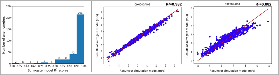
Figure 5. Left - General performance of surrogate model represented as a histogram of R2 scores of the surrogate models of each of the anemometers. Right - Example of performance of surrogate model of two of the anemometers considered. Predictions of surrogate models compared against result of the simulations.

7. Calibration Results

The calibration improved the model’s ability to match real system behavior. Figure 6 illustrates this improvement under conditions without mechanical ventilation, showing how the calibrated model more accurately captures both the magnitude of air velocity and its dependence on traffic flow (piston effect). At a global scale, Figure 7 shows the reduction in prediction errors across anemometers after calibration, confirming the enhanced agreement between simulated and measured airflow. These results demonstrate that the calibrated model reliably reflects the aerodynamic behavior of the system.

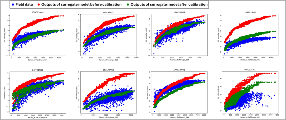
Figure 6. Air velocity (m/s) for different anemometers against the traffic flow (vehicles/hour) in the tunnel segment where the anemometer is placed. Three data sets are represented for each anemometer, field data (blue dots), outputs of surrogate model before calibration (red dots), and outputs of surrogate model after calibration (green dots).

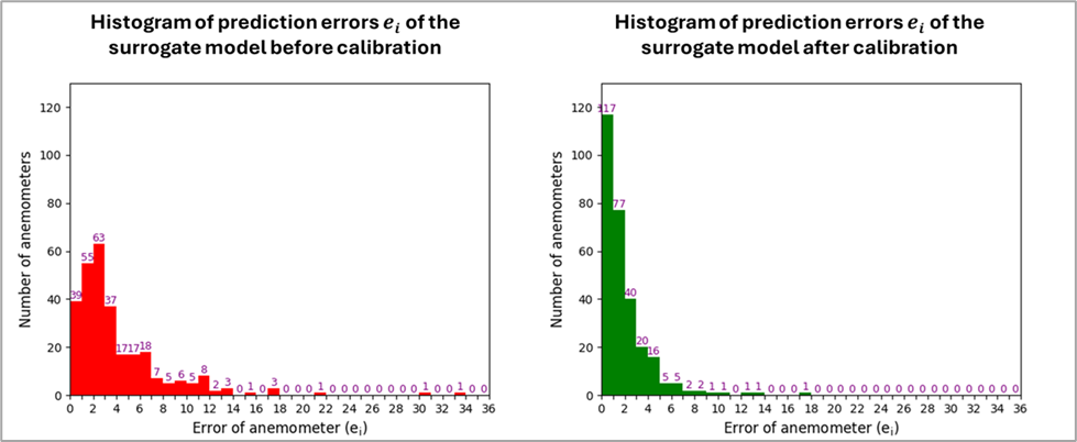
Figure 7. Histograms of the distribution of errors of the surrogate model in the prediction of field data. Left – Before calibration. Right – After calibration.

8. Validation Under Mechanical Ventilation

A second validation phase addressed mechanical ventilation. In this case, the calibrated model was evaluated using controlled on-site tests involving the activation of jet fans and extraction shafts. These scenarios were simulated and compared with the corresponding measured airflow responses. Agreement was strong, with only minor adjustments required to fan efficiencies and shaft parameters. This confirmed that a model calibrated under natural-ventilation conditions can also accurately represent mechanically driven airflow.

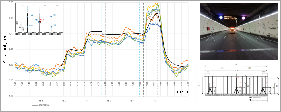
Figure 8. Results of air velocity results obtained in one of the aerodynamic tests. Comparison of simulation results (10NC62AI01 line) with the measurements of the six anemometers used in the test (T1-1, T2-1, T3-1, T1-2, T2-v, T3-2).

9. Application to Ventilation Strategies

After calibration, the model was used to evaluate a wide range of ventilation strategies by simulating different equipment activation scenarios. These simulations provided the basis for defining updated operational algorithms for both fire and sanitary ventilation.

For fire ventilation, the strategies developed aimed to limit the area affected by smoke, prevent spread into adjacent tunnels or branches, and maintain adequate upstream airflow to preserve stratification and avoid backlayering. The calibrated model allowed evaluating these objectives under different fire scenarios to determine the most effective combinations of ventilation equipment for each fire scenario analyzed.

For sanitary ventilation, referring to the control of pollutants generated by day-to-day traffic, the model helped identify equipment configurations capable of maintaining acceptable air quality while optimizing energy use. By exploring many combinations of jet fans and shafts, the model clarified where ventilation is truly needed and where it can be reduced without compromising environmental conditions.

These results have been used to define the ventilation algorithms that will be implemented in the M30 control center. Their performance will be evaluated through full-scale aerodynamic and smoke tests in upcoming project phases.

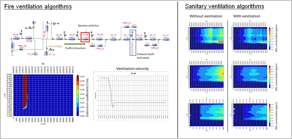
Figure 9. Left - Example of a fire ventilation calculation (fire located in tunnel segment XC_08) performed using the calibrated 1D model. Diagram (top); smoke propagation along the tunnels (bottom left); ventilation velocity (bottom right). Right - Example of a sanitary ventilation calculation performed using the calibrated 1D model. Representation of evolution of NO₂ concentration along three tunnels NC, XC, and FL.

10. Conclusions

Physical models inevitably contain uncertainties in their parameters and assumptions, and these uncertainties become particularly significant in systems with many interconnected elements and large numbers of parameters. Calibration is therefore essential to obtain a robust and reliable model that reflects real behavior. For a system as extensive and complex as the M30 tunnel network, where airflow is influenced by numerous interacting components, meeting this challenge required a methodology combining physical modeling, surrogate-based optimization, and AI-driven data analysis.

The high dimensionality of the parameter space made direct calibration computationally infeasible. This difficulty was overcome by developing a surrogate model capable of reproducing the 1D simulation’s behavior with drastically reduced computation time. This approach enabled efficient exploration of the parameter space, making an iterative optimization process, otherwise unmanageable, viable within real project constraints. The result is a calibrated digital twin that accurately represents system behavior and provides a solid foundation for designing ventilation strategies. The ability to complete this process within realistic time and resource limits demonstrates the practical applicability of the methodology beyond academic contexts.

More broadly, the work highlights the value of integrating engineering expertise with data-driven methods. As tunnel infrastructures become more instrumented, such approaches could support future advances in model calibration, operational optimization, and fire-safety planning. This analysis was made possible thanks to the historical data recorded by the M30 control center, emphasizing the importance of equipping infrastructures with appropriate sensor instrumentation and ensuring that measurements are reliably stored for long-term use.

Methodologies that blend physical modeling with surrogate models and AI techniques offer a promising path for the evolution of fire-safety engineering in complex infrastructures. By enabling models that are both computationally efficient and tightly anchored to real system behavior, they provide practitioners with powerful tools to support design decisions, improve operational strategies, and strengthen resilience across modern tunnel networks.

References

[1] Sanz, J. M., De Kluijver, F., López de Arriba, A., Berges, J., Martínez, M., & Peris, G. (2024). Application of AI to the 1D Ventilation Analysis of a 43 km Complex Road Tunnel Network: Madrid Calle30. In: Proceedings of the 12th International Conference on Tunnel Safety and Ventilation. Graz, Austria: Graz University of Technology.

[2] De Kluijver, F., López, A., Sanz, J. M., Peris, G., Berges, J., & Martínez, M. (2025). Application of Machine Learning for Surrogate Modeling: Calibration of a 1D Ventilation Model of a Complex Road Tunnel Network. NAFEMS Benchmark Magazine, July 2025.

[3] SciPy, "scipy.optimize.differential_evolution — SciPy v1.12.0 Manual." [Online]. Available: https://docs.scipy.org/doc/scipy/reference/generated/scipy.optimize.differential_evolution.html. Accessed: June 11, 2025.

[4] F. Pedregosa, G. Varoquaux, A. Gramfort, et al., "Scikit-learn: Machine learning in Python," J. Mach. Learn. Res., vol. 12, pp. 2825–2830, 2011.

[5] Scikit-learn, "1.11. Ensembles: Gradient boosting, random forests, bagging, voting, stacking." [Online]. Available: https://scikit-learn.org/stable/modules/ensemble.html#gradient-boosting. Accessed: June 11, 2025.

[6] Equa Simulation AB, IDA-Tunnel for Rail and Metro Tunnels. [Online]. Available: https://www.equa.se/en/tunnel/ida-tunnel/rail-metro-tunnels. Accessed: June 11, 2025.

[7] P. Sahlin, L. Eriksson, P. Grozman, H. Johnsson, and L. Ålenius, 1D Models for Thermal and Air Quality Prediction in Underground Traffic Systems, Equa Simulation AB, Sweden.

[8] P. Särkkä, Tunnelling Market in Finland, Chairman, Scientific Committee, WTC2011, Helsinki, Finland.